Your first analysis

Analyse a homogeneous slope from start to finish, in about ten minutes.

This tutorial uses the example model that every new project starts with: a homogeneous slope, 10 m high, from a published benchmark (ACADS problem 1(a), Giam & Donald 1989). You look at its geometry and material, run the analysis, read the result and export it.

1. Start a new project

Start cSlope, or choose File › New. The project contains one model, T-ACADS Simple, shown on the canvas in edit mode.

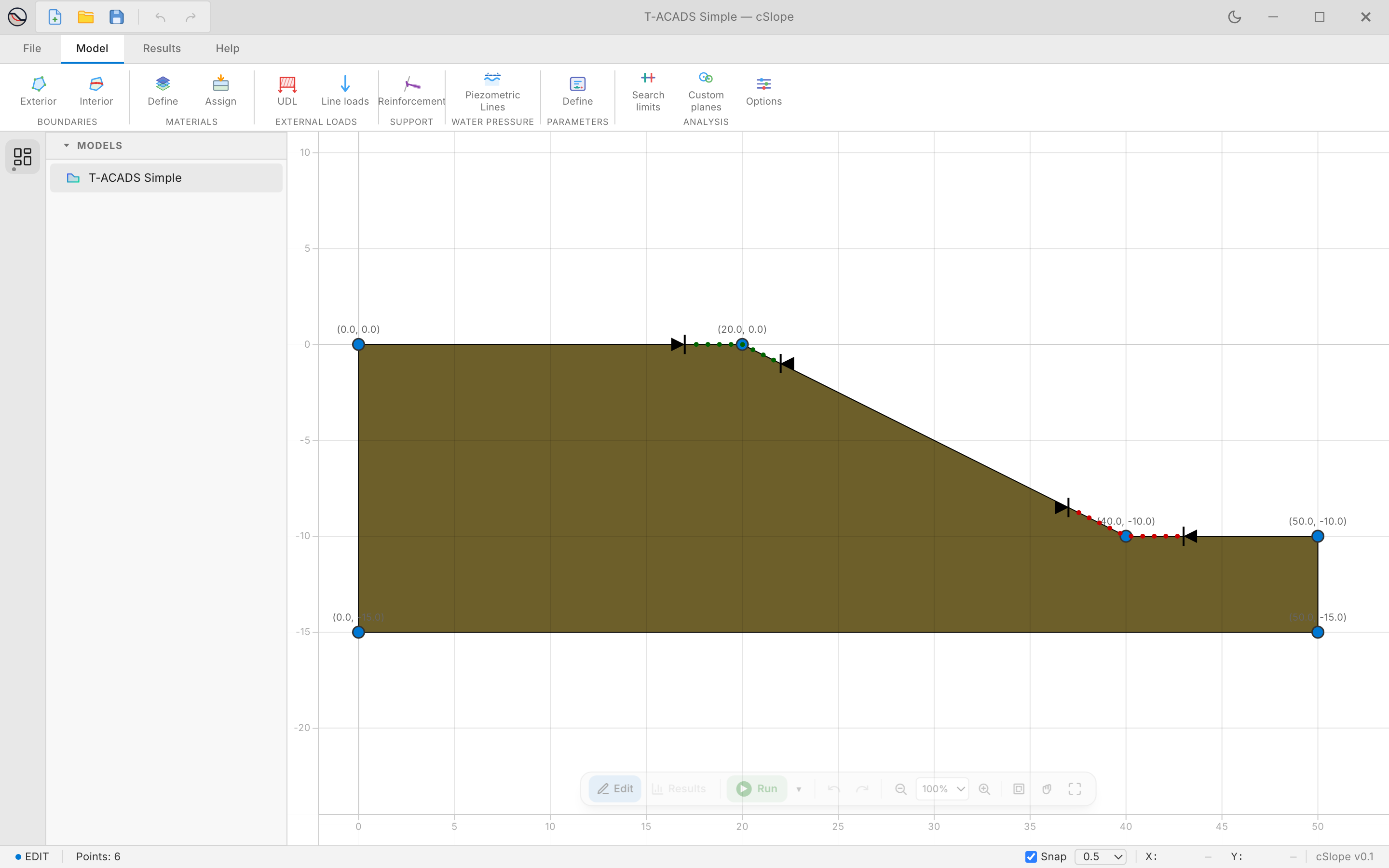
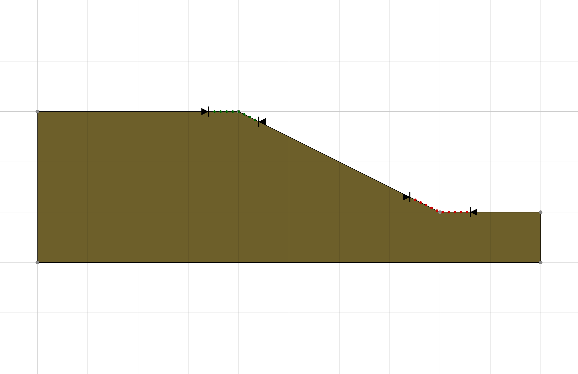
The cSlope window in edit mode with the Model tab open and the example slope on the canvas — The cSlope window: the Model tab of the ribbon, the Explorer with the model, the canvas and the status bar.

The slope has its crest at y = 0 and its toe at y = −10, with a 1V:2H face between x = 20 and x = 40. The soil is one Mohr-Coulomb material.

2. Look at the geometry

Open Model › Boundaries › Exterior. The window lists the points of the exterior boundary. Click a row and the point is highlighted on the canvas. Drag a point on the canvas and watch its coordinates change in the table, then undo with Ctrl+Z.

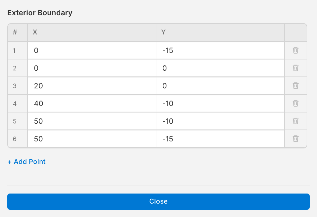
The Exterior Boundary window with six points — The exterior boundary: six points around the section.

The top of the boundary is the ground surface; slip surfaces start and end on it.

3. Check the material

Open Model › Materials › Define. The model has one material, M1: Mohr-Coulomb with γ = 20 kN/m³, φ = 19.6° and c = 3 kPa.

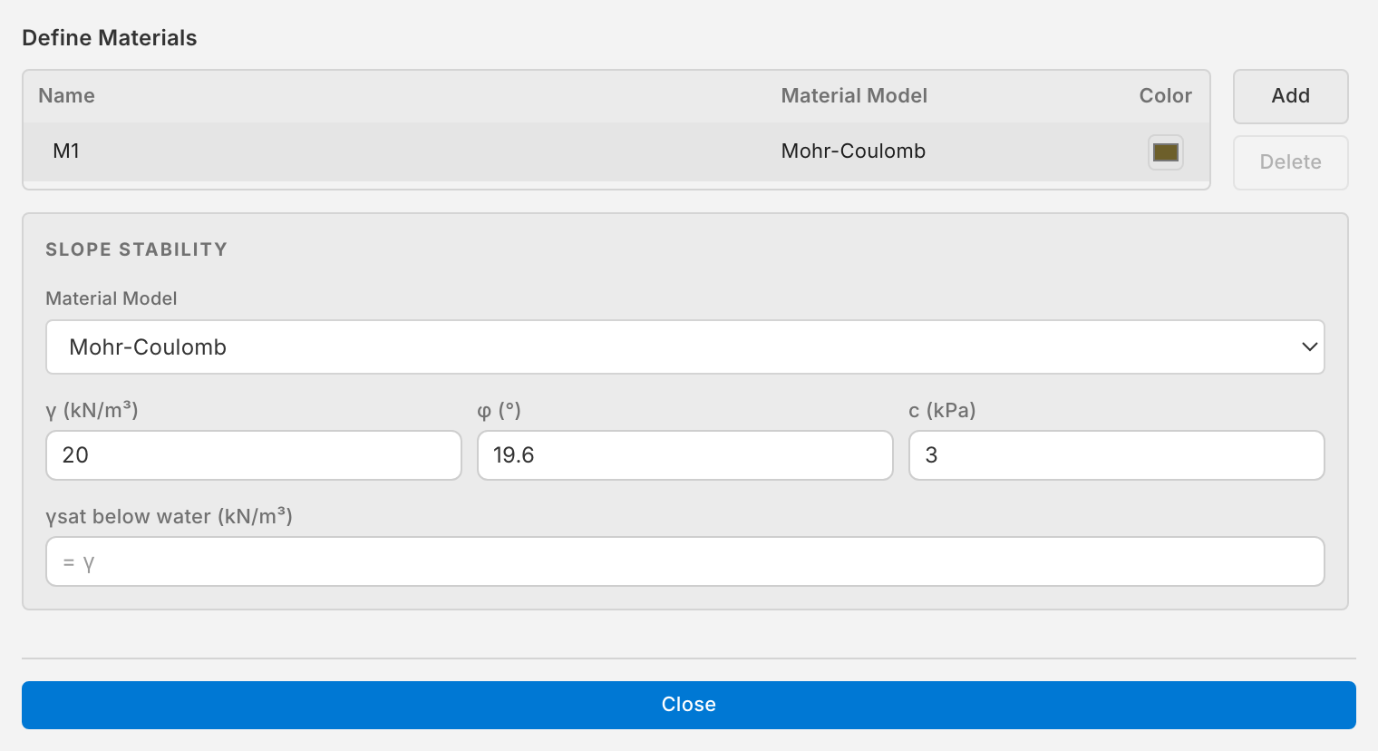
The Define Materials window with material M1 — Define Materials: the material list at the top, the selected material's properties below.

Any change you make applies at once. Leave the values as they are to compare your result with the published one below.

4. Set where surfaces may start and end

Open Model › Analysis › Search limits. Restrict entry/exit ranges is ticked: slip surfaces enter the ground between x = 17 and 22, at the crest, and leave it between x = 37 and 43 at the toe.

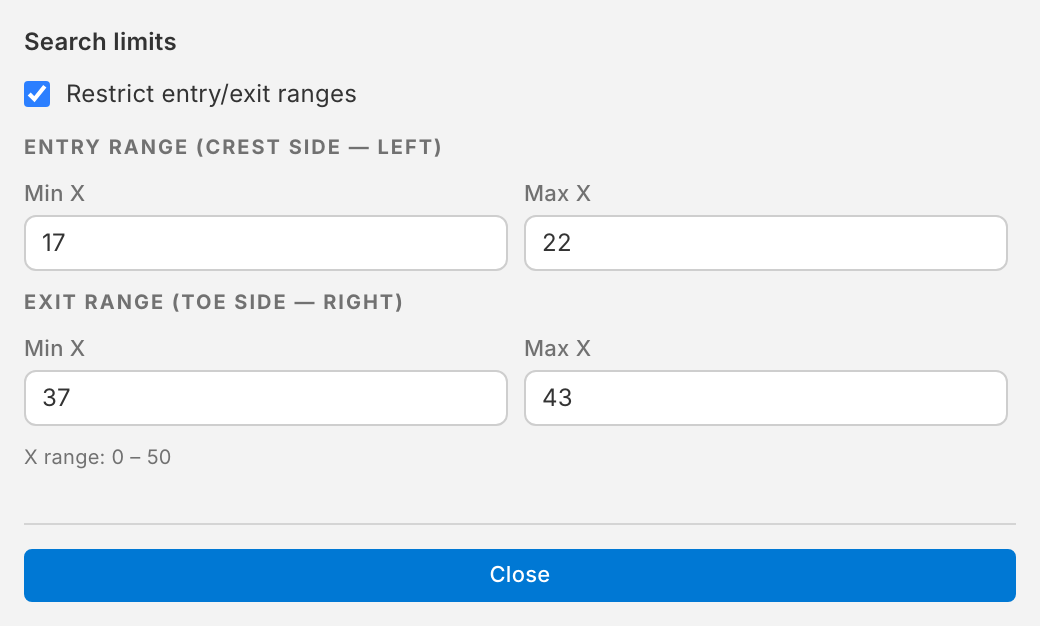
The Search limits window with entry and exit ranges — The entry and exit ranges.

With the window open, the ranges show as markers on the canvas, and you can drag them.

The slope with the entry range on the crest and the exit range at the toe marked — The entry range (green) on the crest and the exit range (red) at the toe.

5. Choose the method

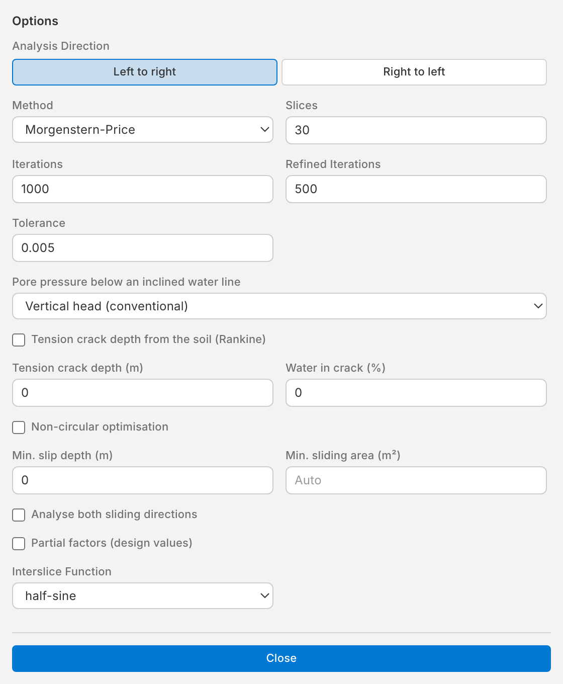
Open Model › Analysis › Options. The method is Morgenstern-Price with a half-sine interslice function and 30 slices.

The Options window — The analysis options.

6. Run the analysis

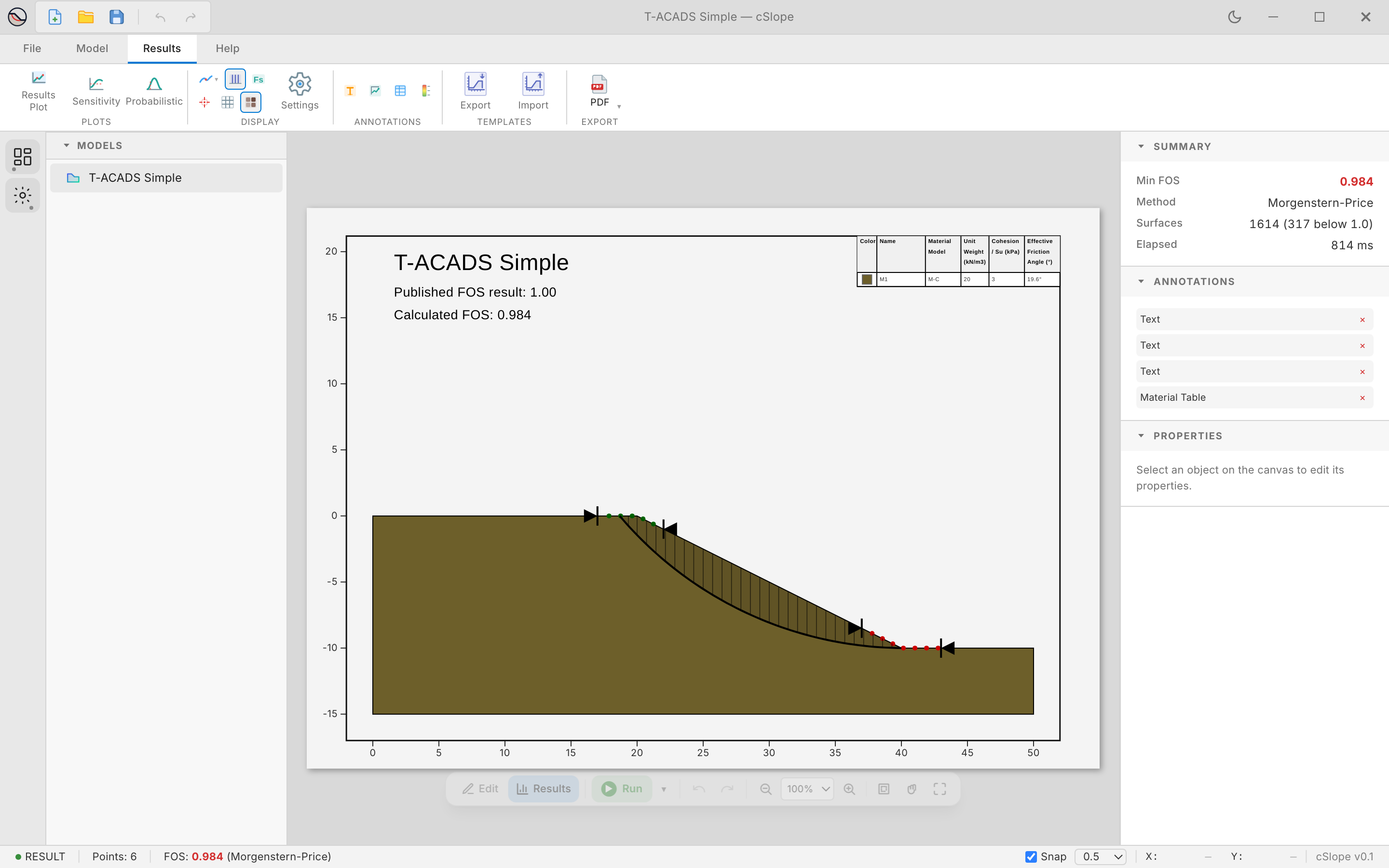
Click ▶ Run on the floating toolbar at the bottom of the canvas. After a moment the canvas switches to result mode.

Result mode with the critical slip circle, the result summary on the right and the Results tab open — The result: the critical circle with its slices, and the summary on the right.

7. Read the result

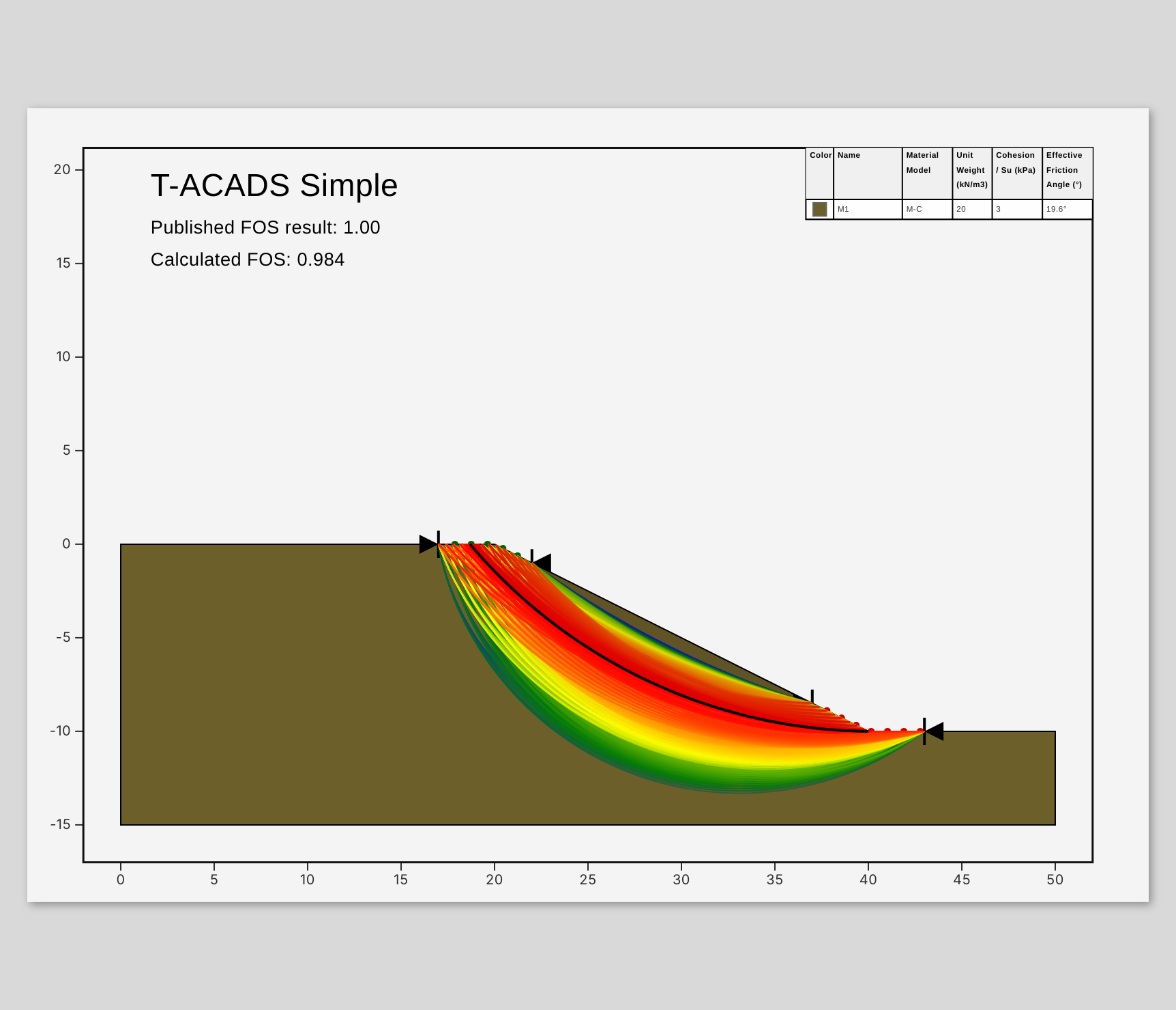
The summary on the right shows a Min FOS of 0.984, found among some 1600 analysed surfaces. The referee answer published for this problem is 1.00; the factor of safety from Morgenstern–Price and similar methods is 0.98 to 0.99.

Choose Results › Display, then All surfaces in the surfaces list, to see every analysed surface coloured by its factor of safety:

All analysed slip surfaces coloured from red to blue by factor of safety — All surfaces, from red (lowest factor of safety) to blue.

Switch back to Critical only.

8. Compare methods

Click Edit, open Model › Analysis › Options, choose Bishop and run again. For a circle in a homogeneous slope, Bishop's value is very close to Morgenstern–Price's (0.985). Janbu gives a lower value; tick Apply correction factor f0 to apply Janbu's correction.

9. Export and save

Choose Results › Export › PDF to save the result sheet as a PDF. The title on the sheet comes from the model's properties: right-click the model in the Explorer and choose Properties to change it.

Save the project with File › Save. The file contains the model and its result.

A slope with a water table.